INTRODUCTION
Climate change and variability have substantial impact on the ecological niches in which many infectious diseases develop, resulting in increased incidence of vector-borne diseases.[1] Epidemics of such diseases cause substantial human and economic losses. Models for predicting vector population increases and ensuing public disease outbreaks could be used in public health surveillance to anticipate and prevent such epidemics and associated substantial human and economic losses.
Risk factors for vector-borne infectious disease have been classified as micro- and macrodeterminants.[2] Microdeterminants are those related to host, disease agent, and vector (suitable conditions for vector proliferation foci, adult female density, etc.).[2] Macrodeterminants could be environmental in nature (latitude, altitude, temperature, relative humidity) or socioeconomic (population density, unplanned urbanization, etc.). Climate elements such as temperature and atmospheric humidity have been linked to the biology and density of breeding foci of Aedes aegypti (NFAe).[3–12] However, most studies have dealt with different factors separately and not examined the issue as a complex whole or addressed variability using an indicator specifically designed for that purpose.
Aedes aegypti (Linnaeus) is one of the main species of mosquito in urban areas. It is native to Africa but has become distributed and adapted to tropical and subtropical regions of the world.[13] Besides being a public nuisance, this mosquito is very important from an epidemiological point of view because it transmits various arboviruses, such as those causing yellow fever, dengue and Chikungunya.[14,15]
Vector-borne disease burden Climate change and variability are shortening the reproductive cycle of vectors of medical importance, such as mosquitoes transmitting dengue, malaria, equine encephalitis, West Nile encephalitis, and other diseases. They grow more easily in humid weather and intense heat, and sometimes they expand their areas of influence, as is the case with Aedes aegypti, when improperly stored water or poor environmental hygiene practices create breeding sites.[16,17] Other vectors known to exist in Cuba are Anopheles albimanus (which can transmit malaria) and Culex quinquefasciatus (which can transmit encephalitis).[18,19]
Cuba’s weather and climate favor year-round vector proliferation. The distribution of adult vector populations (such as Aedes aegypti) in tropical environments varies with the seasons. In the case of Cuba, it is associated with the cycle of rainy and dry seasons. Water conservation efforts in prolonged dry seasons increase the number of larval habitats and, consequently, adult density.[20,21]
Recent scientific and technological advances provide an opportunity to integrate weather predicting ability into health programs. Different modeling approaches are advanced for predicting dispersion and transmission of dengue cases, exemplifying a disease influenced by climate change. Few studies, however, have explored simulation and modeling of the transmitting vector using climatic variables outside the laboratory[22] and incorporating climate variability indicators,[23,24] using entomological indicators with a view to reducing disease outbreaks.[20,21]
Use of climate forecasting for health surveillance It is necessary for the health sector to understand and quantify the specific effects of climate variability and how it contributes to disease burden. Typically, decisionmakers do not fully understand how climate information can be effectively used by the public health sector. Data should be prepared from a health sector perspective and oriented to specific needs (both geographically and in timeliness) to ensure opportune identification of risks.
Interest in using such climatic predictors in health surveillance dates back to the early nineteenth century[25] and has since been a burgeoning line of research, especially in the 1990s.[26–33] However, despite enormous efforts by the scientific community, particularly the work done by Fuller in 2009,[34] much remains to be done.
Developing better predictive models using climate data can strengthen early warning systems and create new climate prediction products to support timely decisionmaking and public health protection. Cuba has been working on this issue for over three decades,[35–44] conducting research leading to the development and strengthening of climate-based early warning systems for human health.
Approaches to climate-based health prediction models Scientists working to provide climate information applicable to the health sector can use statistical or biological approaches. The statistical approach attempts to establish relationships between population-level health indicators and environmental predictors (assuming that the conditions on which such relationships are based will continue in the future). The biological approach focuses on the actual disease transmission processes and the details of all the parameters involved in transmission.[26] It is not a question, however, of choosing one approach over the other since biological approaches are better suited for developing models based on intrinsic factors (susceptibility, infection, immunity, etc.), whereas statistical models are better suited for exploring extrinsic (environmental) factors. Accordingly, a statistical model was developed that would reflect the interaction of extrinsic factors with the health indicator by examining its distribution and spatial variation.[26]
Cuba, a tropical country, is also subject to climate change and variability, and the effects of the latter on the distribution of vectors, particularly Aedes aegypti. Fluctuations that have been taking place in the dry and rainy seasons have brought about substantial seasonal variations in disease patterns, as, for instance, in respiratory diseases.[24,45–47] A similar situation may be occurring in populations of vectors such as Aedes aegypti. Cuba is not immune to the threat of dengue. Aedes aegypti is permanently established in most areas, and this, together with frequent travel between Cuba and countries where dengue is endemic, increases the likelihood of dengue outbreaks.
The foregoing provided the impetus for studying spatial distribution patterns of NFAe and their relation to climate anomalies, and the development of climate-based spatial prediction models for Aedes aegypti that would complement Cuba’s current surveillance system. Included would be predictions of abnormal climate variability from climate indices developed for such purposes,[48,49] to devise NFAe prognostic models that would enable informed decisionmaking. This research study aims, then, at demonstrating the usefulness of climate information for vector surveillance in Cuba, using spatial models for prediction and early warning of NFAe.
METHODS
Design An ecological study was conducted using retrospective and prospective time series analyses, considering the following indicators:
Climate Data from 56 meteorological stations of the Meteorological Institute of Cuba’s climate network were obtained for the main climatic variables, for the period 1981–2013, using the 1981–2010 period for model fitting and 2011–2013 for validation and forecast. Monthly series of dissolved oxygen density in air (g/m2), mean maximum and minimum air temperatures (°C), mean air temperature oscillation (°C), mean relative air humidity (%), mean water vapor pressure (mmHg), mean insolation (hours of sunlight), mean global solar radiation (MJ/m2), mean atmospheric pressure at sea level (hpa), total precipitation (mm) and number of days with precipitation ≥0.1 mm, from which the Bultó climatic indices are calculated: IBt,1,c (Bultó-1), describing monthly and seasonal variation, includes dissolved oxygen density in air, maximum and minimum mean temperature, precipitation, atmospheric pressure, vapor pressure, and relative humidity. IBt,2,c (Bultó-2), describing seasonal and interannual variation, includes thermal oscillation, number of days with precipitation, and solar radiation and hours of sunshine (factors that affect temperature and humidity).[48]
Entomological indicator Infestation index of Aedes aegypti (number of foci), from the database of Cuba’s Ministry of Public Health.
Spatial modeling Identification of spatial patterns and their structure was based on the concept of spatial autocorrelation, the use of exploratory spatial data analysis, calculation of Moran’s I, Moran’s correlograms, and local indicators of spatial association (LISA).[50,51] Areas of hot and cold spots were identified by using a weight matrix determined by the second-order queen contiguity method.[52]
The five fundamental principles governing spatial analysis have been taken into account in this study: interdependence (mutual dependence between different analysis units); asymmetry (gradual concentration and deconcentration in different areas); allotopy (the cause of a spatial phenomenon is often found in a place other than the area under study); nonlinearity; and topology (inclusion of distance variables between two locations, coordinates, densities, etc.).[52]
Spatial autocorrelation This can be represented graphically by Moran’s I correlograms. It implies that the value of a variable is conditioned by the value of the variable in a neighboring region. Vicinity is not necessarily defined as physical contiguity, but there are many criteria to define it, based on a contact matrix. Autocorrelation is positive if regions tend to be geographically close to others of similar values for a variable, i.e., clustered. Autocorrelation is negative if regions with high and low values alternate.[53,54]
Spatial heterogeneity Relationships among spatial epidemiological phenomena vary over the study space, which may occur in two situations: if there is structural instability, when parameters have different values depending on their inclusion in certain areas or not, or if there is error due to model specifications, leading to heteroscedasticity (changing relationships between two variables depending on the value of one of them).
Spatial association measures There are various measures of spatial association, but all originate in the cross-product matrix.[55]
where the Wij matrix is called the contiguity or spatial-weight matrix (its values represent a way of measuring contiguity in the original data). Matrix Cij, on the other hand, is a measure of the proximity of the values i, j, in another dimension (e.g., Euclidean distance, spherical distance, Manhattan distance).[56]
Global association We used Moran’s I[57] in the temporal context, the first measure of spatial autocorrelation in the study of stochastic phenomena distributed in two or more spatial dimensions. For each period t, this statistic is
where Wij is the binary contiguity matrix, such that Wij = 1 if regions i and j have a common border, and Wij = 0 if they do not;[57,58] xit is the value of the observations for each region i in period t (meaning the dry season from November to March; rainy from May to September; and transition in April and October); is the mean for period t, measured in the regions studied;
where n is the number of regions.
This index is analogous to the conventional correlation coefficient, since its numerator is interpreted as the covariance between adjacent units[56] and its values range from +1 (strong positive spatial correlation) to −1 (strong negative spatial correlation).
According to Anselin, a LISA is a statistic that satisfies two requirements: it provides quantification of the degree of important aggregation of similar values around an observation, and the sum of LISAs for all observations is proportional to a global indicator of spatial association.[55] Hence, it is useful to measure the contribution of each observation to the value of global contrast (only in the case of Moran’s I).
Local association Contrasts analyzed in the previous section have a strong limitation: they are not able to consider clustering in a defined area; therefore, lower or higher values would be expected if there was homogeneous distribution.[59]
The local Moran index: considering the purpose of the study, the Moran index adopts the following form for each region i and each period t[58,59]
where
Observations xi,t, xj,t are expressed in differences relative to the mean. The sum regarding j is such that only neighboring regions of i are included, owing to the action of the coefficient Wij, which equals 1 if regions i and j share a border, and 0 if not.
A positive value of ILi,t indicates concentration of similar values, whereas a negative value indicates geographic concentration of different values. To characterize areas of high and low density (NFAe) and their correlations and associations, we used the Moran dispersion scatter plot, with the standardized values of the analyzed variable on the X axis and the lag values on the Y axis. Four types of spatial dependence pattern can be displayed in the graphic, depending on the distribution of observations in its four quadrants. If the values represented are distributed on all four quadrants, there is no spatial autocorrelation. If the point cloud is located around the diagonal running from the first quadrant (upper right end of the graphic: high–high, HH) to the third quadrant (lower left end: low–low, LL), there is positive spatial autocorrelation. When the values represented are located around the diagonal that runs from the second quadrant (lower right end; low–high, LH) to the fourth quadrant (top left high–low, HL), there is negative spatial autocorrelation. Finally, the graphic fits a regression line to the point cloud represented, so that the slope of the regression line coincides with Moran’s I global statistic.[60]
In this way, the exploratory spatial data analysis seeks to identify possible spatial patterns in the data and suggest hypotheses about likely relationships between the variables. Spatial exploratory data analysis is mainly done through visualization of spatial distributions and of associations (using cumulative distribution function, box plot, and Moran’s I correlograms, or LISA).[61]
Formulation of spatial autoregressive models Once the presence of a strong spatial dependence of systemic variables (endogenous and/or exogenous) has been assessed and verified or if there is spatial dependence in the form of disturbances or error,[60] these correlations must be included in the spatial regression model, as was done in this study.
General spatial model This is characterized by dependent variables being correlated spatially as follows:[52–54]
where y is the vector (n × 1) of the dependent variable observations, α is the process level, ρ is the autoregression coefficient, Wy is the vector of independent variables weighted by matrix W of neighboring observations, is a vector of dimensions of the parameters associated with the exogenous variables or regressors (i.e., without spatial lag) in the matrix of dimensions , is the coefficient of the spatial autoregressive structure for error (or heterogeneity), and ε is the sampling error.
Specification of the spatial autoregressive model (SAR) Assuming
in the general model (Equation 6), we have the following expression:
where W1 has the same structure previously defined.
This model differs from the traditional regression in the matrix (I – ρW1)-1, which has a similar form to the Leontief inverse, where â is the vector of its associated coefficients. Therefore, this matrix can be interpreted as follows: the elements outside the main diagonal measure the indirect impact that a variable in an area has over another, whereas the elements of the main diagonal measure the direct plus indirect effect of the variable under study; i.e., if spatial autocorrelation is significant, then when the matrix is multiplied by Xâ, it can be interpreted as the impact of a change in X being not only just â over Y, but that it is transmitted to all geographic units through the indirect effects captured in the inverse matrix, a result that is valid for the following model specification.
If in equation 7 we replace W with the covariance function,
(I − ρC)/σ2, where C is a binary matrix of contiguities, we obtain the conditional autoregressive model.
Spatial error model In this model the dependent variable is not correlated with itself; random sampling error is correlated and its expression is given by:
which is obtained if we assume that:and , in equation 6 where μ is the random sampling error, which follows a spatial autoregressive specification (SAR) with an autoregressive coefficient λ.
Specification of the spatial model For specification of spatial autoregressive models, the strategy described by Moreno was followed.[61] Starting from the basic regression model, initially estimated by the ordinary least squares method, we then incorporated each component until the most plausible spatial model was obtained. These corresponded to mixed spatial regressive models with autoregressive and heteroscedastic errors, depending on the case.[60]
Model goodness of fit There are several indexes or statistics to evaluate how well the model results fit the data. In the study the concordance index Di was used,[62] given by the following equation:
Where: 0 < Di < 1, Pi: prognostic value; Oi: observed value and Ō: mean of the observed values
If Di ≈ 0, it indicates poor agreement between predicted and observed values
If Di ≈ 1, it indicates good agreement between predicted and observed values
Together with this indicator, the skill factor was used, which is given by the following expression:
where, i = 1, 2, . . . , n, Pobs are the actual observations and Pest the estimates from the prediction model, and Var is the variance.[63] Its interpretation is similar to the previous index and also indicates predictive ability.
Theme maps Model results are represented by theme maps that describe the expected spatial distribution of NFAe for each season.
Data processing Moran’s I spatial autocorrelation coefficient was defined for a matrix of neighbors with stations that were in a radius of 20 km, the minimum distance in which all stations had at least one neighbor. The S-Plus 8.1 on Windows and Open GeoDa0.1.4.6-Version 2013 software, developed by Luc Anselin at Arizona State University, the GS-Version 10.0 (GS + Geostatistics for the Environmental Sciences) and ArcGis 10.1 were used to adjust and run models. All variables with p <0.05 were considered statistically significant.
RESULTS
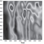
Variation in number of Aedes aegypti foci Seasonal distribution The monthly configuration of NFAe distribution was obtained for each season, based on Cuba’s climate variability pattern. It showed a strong seasonal variation combined with high asymmetry in distribution of its median (Figure 1). A clear trend of increasing foci is evident in recent years, reaching a maximum peak from July and extending through the months of September–November from 2005 to 2010.
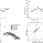
Global and local association Moran’s I correlogramas and values of Moran’s I for the study, detailing the months of January and July (representative of the maximum climate contrasts for the dry and rainy season, respectively), show evidence of a strong positive spatial autocorrelation with lag distances ranging from 1 to 10 km depending on spatial resolution (Figures 2a–d). That means that a significant conglomerate or aggregation of high and low values (positive autocorrelation [I >0]) is present in the area with similar behavior for the rest of the months corresponding to the same season, but with completely different patterns from one season to the other. The largest variations in the index are observed in the months of the rainy season at distances greater than 10 km, where a sign change occurs associated with a disaggregated or dispersed distribution for both climate and vectors, while in the dry season it occurs from 20 km, as shown in the example from January.
Figure 1: Pattern of interannual variation in number of Aedes aegypti foci for the period 1998–2012

Pattern of spatial vector behavior It can be observed that NFAe presents a clear spatiotemporal pattern overall, with a changing spatial pattern by month, analyzed in each of the seasons, with marked spatial heterogeneity, showing areas of increased clusters of high–low values that lead to the presence of clusters (hot and cold spots) in areas close to the populated region (Figures 2b and 2d). This situation is similar when analyzed by month; space limitations make it impossible to show all the figures for all months.
Figure 2: Moran’s I correlogram, dispersion diagram and spatial distribution of Aedes aegypti in risk areas by conditions, Cuba, January (a and b) and July (c and d)

Local association In the Moran scatter plot and Ae scatter map, there is high concentration of points in quadrants I and III, corroborating the presence of a high concentration of similar vector density values (areas with high values surrounded by areas of high values—HH—with areas of low values surrounded by areas of low values—LL) in the study area, as well as strong positive spatial correlation. The dissimilar values (showing spatial heterogeneity) are interesting; they may be associated with the diversity and configuration of the ecological components (biotic and abiotic), which occur with low frequency in quadrants II and IV. In all periods analyzed, but not in all areas studied, this configuration presents highly significant (p<0.05) variations in intensity when passing from a rainy-season month to a dry-season month. (See right side of Figures 2b and 2d).
In all cases the contrast of Moran’s I spatial autocorrelation is clearly significant at the 5% level, rejecting the hypothesis of random distribution of NFAe and therefore reflecting how contiguous regions have similar Aedes density values in general, in addition to a clear majority and significant association of high–high (H–H) and low–low (L–L) values (Figures 2b and 2d).
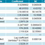
Estimation and model fit In the model results, large differences are observed regarding the variables that explain spatial behavior and its meaning for a month in the dry period (such as January) and for one in the rainy season (such as July); Table 1 shows the attributes of the SAR and conditional autoregressive models for NFAe for the two months. January shows a pure autoregressive spatial model; whereas July, a conditional autoregressive one. Clearly, their parameters are different, although both have a matrix structure with equal weights (W_foci). In July (rainy season), the model structure is centered on variations attributable to spatial heterogeneity and on the seasonal climate variation indicated by Bultó-1, unlike in January, where the model’s structure is explained by autoregressive variations and the influence of the climate variability signal described by Bultó-2, and secondarily on the seasonal variation given by Bultó-1.
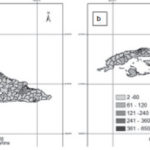
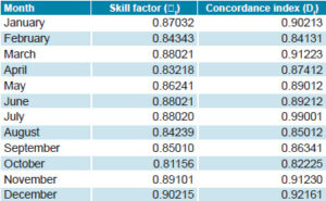
Concordance of actual number of Aedes aegypti foci with model predictions Figure 3 shows the agreement between values obtained from the models and those observed for the month of August 2013. The models’ predictive plausibility is evident; they describe the real behavior and configuration of NFAe spatial patterns. Table 2 shows the quality of the models’ outputs for predicting NFAe spatial distribution by month.
Table 1: Parameters and model fit (SAR and CAR) for number of Aedes aegypti foci, Cuba, January and July

CAR: conditional autoregressive SAR: spatial autoregressive
*rho: spatial autoregressive coefficient
**lambda: spatial error coefficient
Figure 3: Predicted (a) and observed (b) number of Aedes aegypti foci according to climatic variability, Cuba, August 2013

DISCUSSION
Seasonal distribution NFAe distribution shows monthly and seasonal variability in the behavior and distribution of the species due to climatic influence on the density and movement or shift of the population to other months, showing a changing distribution over time, findings similar to those of other authors.[64–66] That is to say, the data suggest a pattern of heterogeneous temporal behavior since there is a contagion effect with different densities and degrees of dispersion by season and year. The largest variations and densities occurred in July–October 2007, whereas in 2008 the period of greatest NFAe density and variability went on until November, with expansion receding in 2009 and 2010, possibly because of the intensity of vector control efforts in those last two years. These variations are significant, despite the Cuban climate’s lack of marked climatic seasonality, with just the two seasons typical of the tropics, rather than the four well-defined seasons of higher latitudes.[17,67,68]
It is clear that effects on the vector habitat (urban, suburban, and rural ecosystems) are due, among other factors, to the influence of climate variations shown by the climatic indices (Bultó-1 and -2) for the months of the rainy season and transition (October–November), combined with other environmental factors (higher number of potential breeding sites) that favor vector growth and reproduction. These characteristics could result from pressure on vector habits and ecosystems by human activity, which, along with other factors, could help to explain high interannual variation.
The months of highest NFAe (September and October) are associated with high humidity, high temperatures and low hours of light (variables included in the Bultó-2 index); this creates a compounding effect. These conditions favor high vector reproductive rates, which could explain the increase observed in that period.[17,64,67–70]
Seasonal and interannual variations of NFAe spatial pattern found in our study, confirm other findings in tropical settings, where populations of vectors are modified both by seasonal and nonseasonal climate variations and by locality.[64,66,68–72]
Table 2: Quality of spatial prediction of number of Aedes aegypti foci, Cuba, 2011�2013

Spatial distribution Strong positive spatial autocorrelation is shown by the Moran’s I values and correlograms for January (dry season) and July (rainy season), with lag distances ranging from 10 to 20 km, depending on spatial resolution; that is, there was strong clustering of high and low values within months in a single season, but slight changes between months from one season to the next. The largest index variations were observed in July, starting at a resolution of 10 km, where a sign change occurs associated with a dispersion pattern, for both climate and vectors. Thus, these findings confirm that NFAe has a spatial structure with strong autocorrelation and a marked seasonal effect.[20]
LISA analysis An important element is the remarkable concentration of point masses in quadrants I and III, with predominance of a spatial concentration of similar values of NFAe. It is characterized by regions of high values surrounded by others with high values, and areas of low values surrounded by others of low values, with a very interesting change in the transition months, where the spatial structure (degree of correlation) is maintained, but not spatial pattern (physical distribution). It shows the influence of climate variability described by the Bultó-1 and -2 indices[29] on NFAe distribution. Therefore, if climate variations are reflected in the spatial distribution, one can expect that, if the climate changes, the spatial distribution of Aedes aegypti foci will also change.[20–24]
It is evident that there are very few areas of discrepancy between a value in a region and the average observed in the neighboring regions, reproducing very well the spatial variations and structures generated by the data.
Significant clusters of Aedes aegypti foci in each of the regions are not randomly dispersed, but are located close together and concentrated in defined areas of Cuba, near the most densely populated areas. Another remarkable feature is that all identified clusters concentrated similar values for study variables; no region showed behavior significantly dissimilar to that shown by its neighbors, displaying a clear overall spatiotemporal pattern, with changing spatial patterns by month and season and marked spatial heterogeneity. This leads to clustering (hot and cold spots) in areas close to the most populous region. This clustering is more marked in rainy-season months.
Model analysis From the correlograms for each of the months, a clear spatial variation with a trend to vector increase can be seen in the most densely populated areas of Cuba (darker regions), which have favorable conditions for vector spread (prevalence of water tanks, containers in dumps and other waste deposits). When this situation is combined with warmer and wetter weather conditions, or when there is widespread drought with unsuitable water-storage practices (variations described by the Bultó indices), rapid colonization of breeding grounds may occur, as previously described.[20,21]
The model’s autoregressive structure represents contagion (rho) between neighbors, where exogenous shocks spread between neighboring units, allowing us to understand the dispersion and configuration of vector populations and lags (distances), the influence of one region over the next, as well as describing the influence of climate variability as a determinant in each region (the spatial lags and the endogenous variable explain the direct relationship between neighboring units). Finally, the lambda component (random error) represents how dispersion attributable to noise occurs on neighboring units in the model, allowing indirect description of spatial structures between neighboring units. This confirms the need to understand both spatial and temporal variability in each region in order to understand vector dispersion, a unique contribution of this study. Other studies take into account only the temporal components and their representation in the form of maps.[19,21–23,30,38]
Our results confirm that the Bultó indices of climate variability are excellent predictors of the spatial distribution of NFAe,[44,49,64,67] and thus are suitable as surveillance indicators, consistent with Fuller’s work on climate and dengue in Costa Rica.[34]
Variable significance between 90% and 95% indicates that there is no reason to reject the hypothesis of no spatial autocorrelation of the errors; that is, the model is robust. Furthermore, the determination coefficient remains above 70%. The fact that the coefficient signs for each model are opposite confirms that negative climate anomalies in the rainy season favor increased populations of Aedes. In the second model, factors are interpreted differently because, when conditions are warmer than expected, with very high humidity values and high variability and heterogeneity (described by lambda, referring to the model’s noise component), they bring about increased vector populations, very typical conditions in our dry winter season.
The high significance and goodness of fit of the models confirms that NFAe’s spatial distribution is not random, but subject to the physical–geographical characteristics of the location, climate variations, and the characteristics of the vector itself, which are reflected adequately in the models proposed.
There are no previous studies using this sort of model to simulate Aedes foci distribution in space and time, using complex climate indices as predictors. Other research has employed linear models, probability distributions or time series,[19,21–23,30,38,44,64] using isolated climatic variables, such as temperature or precipitation), which do not completely describe climate variation. Nor does previous research address changes attributable to projections and variability associated with climate change, as done with our models.[19,20,29,44]
Our work meets Kelly’s recommendations to develop spatiotemporal models and early warning systems based on predicted variables or climate indicators.[66] Mapping predicted NFAe provides decision-makers with easily understandable information about likely vector incidence and spread: the maps indicate municipalities at higher risk of a dengue epidemic, according to spatial distribution of NFAe, a requisite for early warning health surveillance systems.
CONCLUSION
The configuration and spatial structure of NFAe is associated with seasonal variations in climatic variables. The two spatial models obtained for prediction and early warning of increased populations of Aedes aegypti, using complex Bultó indices of climate variability, are suitable for alerting Cuban health authorities to likely vector population changes by season and month, at a resolution of 20 x 20 km. The usefulness of climate information for epidemiological surveillance is thus demonstrated.


